


HPM-2002-OBEVacuum Gauge Page 30 of 39
loss is only approximately 10% of E
s
. If ambient changes are small compared to the absolute values of the
temperature this loss can approximated as a constant with temperature.
Since the first two losses are essentially constant at high vacuum for a given sensor, we can measure these
losses and subtract them from the input power which leaves only the rate of heat transmission through the gas
(E
g
).
In the viscous flow regime, the E
g
loss is directly dependent on the thermal conductivity of the gas (K
g
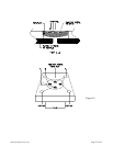
), the
surface area of the membrane, the differential temperature and is inversely proportional to distance between the
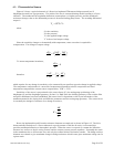
membrane and the lid. It can be written as
E
g
= (K
g
∆T A
s
)/∆x
The thermal conductivity of the gas is essentially constant when in viscous flow where the Knudsen number
(Kn) is less than 0.01. In the viscous flow regime there is no change in sensor output with pressure since all of
the losses are constants with pressure.
In the molecular flow regime where (Kn > 1) the thermal conductivity of the gas becomes directly
proportional to the gas pressure as shown below. We can expect then that E
g
will be constant at high pressures
and directly proportional to the pressure at low pressures. The energy loss, E
g
, changes between these two
controlling equations as the system passes through the transition region (0.01 < Kn < 1).
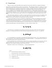
E
g
= a
r
L
t
(273/T
h
)
1/2
(T
h
-T
a
)A
g
P
where
a
r
= accomodation coefficient
L
t
= free molecule thermal conductivity
T
h
= temperature of heated membrane
T
a
= ambient temperature
P = pressure
A
g
= surface area of the heated portion of the membrane
For nitrogen at a pressure of 760 Torr and a temperature of 20 °C the mean free path (λ) is less than 1 x 10
-
7
meters and is inversely proportional to pressure. Since the thermal transfer distance (∆x) is a few micrometers,
this sensor will remain in the molecular flow regime at a much higher pressure (10 Torr) than is typical for a
thermal vacuum gauge. This extends the linear response part of the output curve up into the 1 Torr range. The
nonlinear transition region will extend up to 1000 Torr.
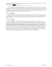
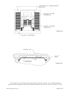
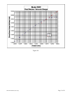
4.4. Dual Sensor Operation
The microprocessor in the control unit continuously monitors the outputs of both the piezoresistive sensor
and the Pirani sensor. Figure 4.4 shows representations of the sensors output over the pressure range from 10
-5
Torr to 10
+3
Torr. The microprocessor uses the output of the piezoresistive sensor at high pressures (>32
Torr) and uses the output of the Pirani sensor at low pressures (<8 Torr). In the crossover region, a software
averaging algorithm ensures a smooth transition between the two sensors.