


IM 01E20C01-01E
6-31
6. PARAMETER DESCRIPTION
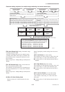
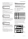
[J20: Flow Direction] Setting of the flow direction
Upon shipment from the manufacturing plant, the
system is setup such that flow in the same direction, as
shown by the direction of the arrow mark on the
flowtube, will be measured as forward flow; however,
this parameter can be used to set “Reverse” so that
flow in the opposite direction to the arrow mark will be
treated as forward.
Note: This function does not apply to measurement in
both the forward and reverse directions, al-
though this can be setup using by selecting
“Fwd/Rev Ranges” from either F10: SO1
Function or .
Setting Function
Forward direction corresponds with arrow mark
Forward direction is opposite to arrow mark
Forward
Reverse
T0638.EPS
[J21: Rate Limit] Setting of the rate limit value
᭹ This parameter is used in situations where sudden
noise cannot be eliminated by increasing the
damping time constant.
᭹ In situations where step signals or sudden noise
signals caused by slurries or the like are entered, this
parameter is used to set the standard for determining
whether an input corresponds to a flow measurement
or noise. Specifically, this determination is made
using upper and lower rate limits and using the dead
time.
᭹ Rate limit values are set using a percentage of the
smallest range. The range of deviation per one
calculation cycle should be input.
[J22: Dead Time] Setting of dead time
This parameter sets the time for application of the rate
limit, and if a value of 0 is set, the rate limit function
will be terminated.
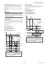
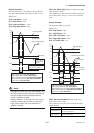
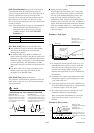
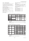
NOTE
Determining rate limit value and dead time
F0616.EPS
T0
T0
2%
2%
Rate limit value:
Determines the level for output
fluctuation cutoff. For example,
if this is set to 2%, noise above
2% will be eliminated as shown
in the diagram.
Dead time (T
0
):
This is to be determined using the
output fluctuation width. If noise
exceeds the dead time as shown in
the diagram below, the dead time
should be made longer.
᭹ Signal processing method:
A fixed upper and lower limit value is setup with
respect to the primary delay response value for the
flow rate value obtained during the previous sam-
pling, and if the currently sampled flow rate is
outside these limits, then the corresponding limit is
adopted as the current flow rate value. In addition, if
signals which breach the limits in the same direction
occur over multiple samples (i.e., within the dead
time), it is concluded that the corresponding signal is
a flow rate signal.
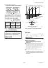
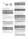
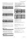
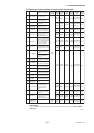
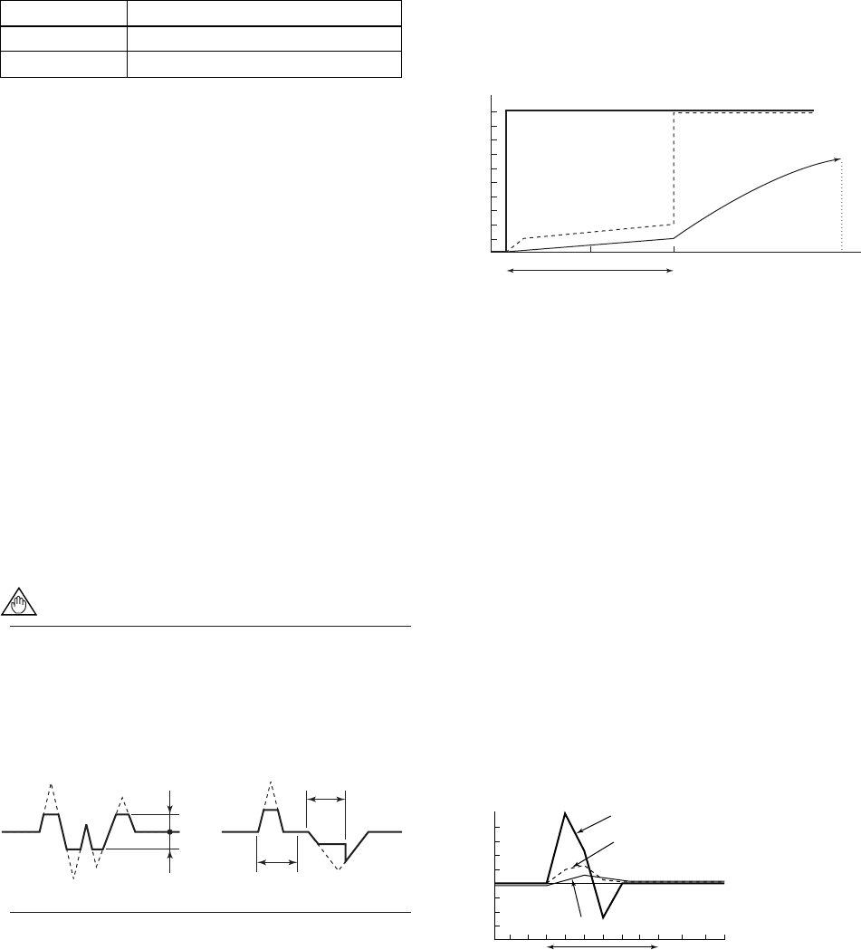
Example 1: Step input
F0617.EPS
10
%
1
%
Step signal
Flow rate value
after rate limit
processing
63.2
%
100 225
Dead time: 3 s
Input: 0 to 10%
Damping time constant: 3 s
Dead time: 3 s
Rate limit value: 1%
Number of signal samples
Flow rate value after
damping
(a)
(b)
(c)
(d)
(1) In comparison with the previous value at (a), it is
determined that the signal is in excess of the rate
limit value and the response becomes 1%. How-
ever, the actual output applies damping, and
therefore the output turns out to be as indicated by
the solid line.
(2) Subsequent flow values within the dead time zone
correspond to signals of post-damping flow value
+ rate limit value (1%).
(3) Since input signals do not return to within the rate
limit value during the dead time, it is determined at
(c) that this signal is a flow rate signal.
(4) The output signal becomes a damped curve and
compliance with the step signal begins.
Three seconds after determination of a flow rate
signal in the above figure, a level of 63.2% is
reached.
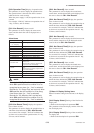
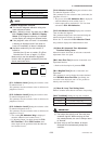
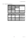
Example 2: Slurry noise
F0618.EPS
+1
%
-1
%
Dead time: 1 s
Flow rate value after damping
Flow rate value
after rate limit
processing
Slurry noise
Input: 0 to 10%
Damping time constant: 1 s
Dead time: 1 s
Rate limit value: 1%
Time
In the figure on the left, it is
determined that the slurries
noise signal is not a flow rate
signal.